DAY21. 주성분분석, 요인분석

주성분분석

01. 고유값과 고유행렬

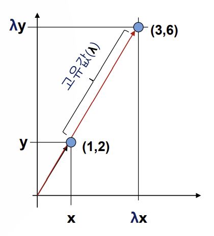
정방행렬A(n, n)에 대해 Av = λv를 만족할 때 (v:0이 아닌 고유 벡터, λ:상수 고유값)

 

* 정방행렬? 같은 수의 행 X 같은 수의 열

* 고유값? 상수(scala)값 λ(람다)

정방행렬A(n, n)를 요약하는 값(=특이값을 나타내는 값)

행렬에서 차원(열:변수)의 특징

수치의 크기는 특징의 강도

* 고유벡터? 고유값에 해당하는 0이 아닌 벡터

* 응용분야 : PCA(주성분분석), SVD(특이값분해), Pseudo-Inverse(유사 역행렬), 선형연립방정식 등

 

 

선형결합-선형변환

선형변환? n차원의 행렬A를 벡터v와 곱하여(선형결합하여) 1차원의 다른 벡터Av로 변환(축소)

행렬곱 수식 : Av = A %*% v

[예] Y = a1X1 + a2X2 + … +anXn

y = 1*3 + 2*0 = 3

y = 1*8 + 2*(-1) = 6

 

 

고유값과 고유벡터

선형변환에 의해 만들어진 Av를 벡터v로 만들기 위해서 λ=3 지정할 때, 다음 식이 성립

 

λ = 3 (행렬A의 고유값)

Av == λv (v : 행렬A의 λ에 대한 고유벡터)

 

* 벡터v를 행렬A로 선형변환 시킨 결과, Av가 벡터v의 상수(λ)배가 성립 될 때 고유벡터 존재

 

 

고유값과 고유벡터 관계

고유벡터(v) : 방향은 유지되고, 크기만 변화되는 방향벡터

고유값(λ) : 고유벡터의 변화되는 크기(scale)

 

 

 

 

 

02. 주성분분석 vs 요인분석

공통점	차이점
변수 축소 기능 : 상관관계가 있는 변수들을 선형결합	변수 통합 기준 • 주성분분석 : 수치적인 상관성을 기준으로 변수 통합 • 요인분석 : 개념적/논리적인 상관성을 기준으로 변수 통합
데이터 패턴 탐색 : 주성분/요인을 통해서 변수 특성 이해	변수 축소의 목적과 생성된 변수 개수 • 주성분분석 : 탐색적 관점으로 보통 2~3개 • 요인분석 : 확인적 관점으로 주어진 상위 요인의 수
다른 분석을 위한 사전분석 : 회귀분석에서 독립변수 간 다중공선 성이 존재하는 경우 상관성이 높은 변수를 주성분/요인으로 축소	변수 간의 중요도 • 주성분분석 : 제1주성분이 분산 변동량 가장 많이 가지고 있음(중요한 변수) • 요인분석 : 변수들의 중요도는 대등한 관계
입력변수 : 회귀분석, 군집분석, 시계열분석 등에서 입력변수 사용

 

 

 

 

 

 

03. 주성분분석

다변량 자료 대상 수치적 상관성이 있는지 관찰, ‘주성분’ 통합

모든 변수들의 공통적인 선형변화를 통해 상관성 있는 변수들 간의 정보 단순화

보통 2~3개 정도 성분 추출, 제1주성분의 변화량(설명력)이 가장 크다. (중요도가 가장 큼)

주성분의 누적변화량 85%정도 이상이면 주성분으로 도출

 

 

다변량 자료 분석

다변량 자료? 둘 이상의 서로 상관관계에 있는 변수들을 포함하고 있는 자료

주성분분석은 다변량 자료분석 방법 중 하나

 

 

주성분분석 필요성

1) 차원의 저주? 차원이 증가함에 따라(=변수의 수 증가) 모델 성능이 안 좋아지는 현상

2) 다중공선성(Multicollinearity) : 한 독립변수의 값이 증가할 때 다른 독립변수의 값이 이와 관련하여 증가하거나 감소하는 현상 (회귀분석 결과 왜곡)

3) 과적합(Overfitting) : 학습데이타에 대해서는 오차가 감소하지만 실제 데 이타에 대해서는 오차가 증가하는 현상

4) 성능저하 : 모델링 과정에서 저장공간과 처리시간이 불필요하게 증가

 

 

선형변환

여러 변수들을 대상으로 가중결합 시킨 형태

n차원의 정보를 가중치 a와 곱하여 1차원으로 축소하는 연산 과정

 

 

데이터 표준화

주성분분석은 측정 단위에 따라서 분산이 크게 달라짐

표준화 하는 경우	표준화 하지 않는 경우
측정 단위가 다른 경우 상관행렬로부터 시작하는 주성분분석	자료의 단위가 동일한 경우 분산공분산 행렬로부터 시작하는 주성분분석
ex. 변수 중 하나는 cm, 다른 하나는 kg인 경우 ex. 다른 한 변수는 1자릿수, 다른 변수는 3자릿수인 경우	변수의 단위 그대로, 변동 그대로 사용하기 때문에 데이터와 모집단의 특성을 잘 드러낼 수 있다.

 

 

주성분분석 단계

데이터 특성 파악 : 상관분석으로 변수 간 관계 파악

가중계수 추출 : 상관계수 행렬의 특징을 가지고 있는 고유값과 고유벡터 추출

차원축소 : 표준화된 데이터셋 대상으로 주성분 분석

주성분 판정 : 주성분 개수 판정 및 입력변수 생성

 

[실습]
실습 목적 : 6개 과목의 특징을 대상으로 주성분분석 수행 -> 유사 과목 파악    
변수 설명 : 6개 과목에 대한 10개의 특징 수치화(5점 척도) 
s1 : 자연과학, s2 : 물리화학
s3 : 인문사회, s4 : 신문방송
s5 : 응용수학, s6 : 추론통계

s1 <- c(1, 2, 1, 2, 3, 4, 2, 3, 4, 5)
s2 <- c(1, 3, 1, 2, 3, 4, 2, 4, 3, 4)
s3 <- c(2, 3, 2, 3, 2, 3, 5, 3, 4, 2)
s4 <- c(2, 4, 2, 3, 2, 3, 5, 3, 4, 1)
s5 <- c(4, 5, 4, 5, 2, 1, 5, 2, 4, 3)
s6 <- c(4, 3, 4, 4, 2, 1, 5, 2, 4, 2)
name <-1:10

dataset 가져오기 : 1차(iris), 2차(data.frame)

dataset <- data.frame(s1, s2, s3, s4, s5, s6)
dataset
str(dataset) # 'data.frame': 10 obs. of  6 variables:

[단계1] 데이터 특성 파악 : 변수의 상관성 분석 

cor(dataset) # 상관계수행렬(정방행렬)

         s1          s2         s3         s4         s5         s6
s1  1.00000000  0.86692145 0.05847768 -0.1595953 -0.5504588 -0.6262758
s2  0.86692145  1.00000000 0.06745441 -0.0240123 -0.6349581 -0.7968892
s3  0.05847768  0.06745441 1.00000000  0.9239433  0.3506967  0.4428759
s4 -0.15959528 -0.02401230 0.92394333  1.0000000  0.4207582  0.4399890
s5 -0.55045878 -0.63495808 0.35069667  0.4207582  1.0000000  0.8733514
s6 -0.62627585 -0.79688923 0.44287589  0.4399890  0.8733514  1.0000000
* s1:s2, s3:s4, s5:s6 상관성 높음 


[단계2] 가중계수 추출 : 고유값과 고유벡터 : chap12_1_Eigenvalue 참고 
고유값(λ)  

en <- eigen(cor(dataset)) # 상관계수행렬 -> 고유값,고유벡터    
names(en) # "values"  "vectors"

en$values # $values : 고유값 보기(변수 개수와 일치)

# 3.44393944 1.88761725 0.43123968 0.19932073 0.02624961 0.01163331
* - 고유값이란 어떤 행렬(상관관계수 행렬)로부터 유도되는 특정한 상수값

고유값 전체합 = 총분산 

sum(en$values) #6

각 분산의 비율 = 고유값 / 총분산 

en$values / sum(en$values)

0.573989906 0.314602874 0.071873280 0.033220121 0.004374934 0.001938885
0.573989906 + 0.314602874  # 0.8885928
0.573989906 + 0.314602874 + 0.071873280 # 0.9604661

en$vectors # 고유벡터

           [,1]         [,2]        [,3]       [,4]        [,5]        [,6]
[1,] -0.4062499 -0.351093036  0.63460534  0.3149622  0.45699508  0.03041553
[2,] -0.4319311 -0.400526644  0.11564711 -0.4422216 -0.57042232  0.34452594
[3,]  0.2542077 -0.628807884 -0.06984072  0.3339036 -0.35389906 -0.54622817
[4,]  0.3017115 -0.566028650 -0.37734321 -0.2468016  0.50326085  0.36333366
[5,]  0.4763815  0.008436692  0.58035475 -0.6016209  0.05643527 -0.26654314
[6,]  0.5155637  0.021286661  0.31595023  0.4133867 -0.28995329  0.61559319

plot(en$values, type="o") # 고유값을 이용한 시각화(elbow point 기준)

[단계3] 차원축소 : 주성분분석 
상관계수를 적용한 고유벡터와 관측치 간의 선형결합 : dataset의 상관계수행렬을 이용하여 주성분분석 수행   

PCA <- prcomp(dataset, center = TRUE, scale. = TRUE) # 변수들의 단위가 다른경우 적용  
# center = TRUE, scale. = TRUE -> 평균=0, 분산=1

 

PCA # 주성분의 분산과 회전값

Standard deviations (1, .., p=6): 표분편차(분산) = 고유값 제곱근 
1.8557854 1.3739058 0.6566884 0.4464535 0.1620173 0.1078578

sqrt(3.44393944) # 1.855785

# Rotation (n x k) = (6 x 6): 고유벡터 부호 회전 

주성분분석의 속성  

names(PCA) # "sdev"     "rotation" "center"   "scale"    "x"   
# sdev, rotation, x 속성이 중요함

1) 각 주성분의 분산

PCA$sdev # 1.8557854 1.3739058 0.6566884 0.4464535 0.1620173 0.1078578

 

2) 각 주성분의 Rotation 값 

PCA$rotation

3) x : 주성분 점수 

str(PCA$x) # num [1:10, 1:6] -> [관측치, 변수]

PCA$x

round(PCA$x[,1:3],2)

#         PC1        PC2        PC3
#[1,] -1.2195113 -2.0459190  0.2058941
#[2,] -0.8619728  0.4960040  0.0733061
#[3,] -1.2195113 -2.0459190  0.2058941
#[4,] -1.3831687 -0.3387559 -0.3876923
#[5,]  1.5989191 -0.7852011  0.3581558
#[6,]  2.5004922  0.9502748  0.8197018
#[7,] -2.7991446  1.8549340  0.1375841
#[8,]  1.4637914  0.6653457  0.6438323
#[9,] -0.5785476  1.6426768 -0.6461737
#[10,]  2.4986537 -0.3934403 -1.4105023


[단계4] 주성분 개수 결정 

summary(PCA) #주성분 분석에 대한 결과 요약 설명

#Importance of components:
#                         PC1    PC2     PC3     PC4     PC5     PC6
#Standard deviation     1.856 1.3739 0.65669 0.44645 0.16202 0.10786
#Proportion of Variance 0.574 0.3146 0.07187 0.03322 0.00437 0.00194
#Cumulative Proportion  0.574 0.8886 0.96047 0.99369 0.99806 1.00000

* Standard deviation : 표준편차 
* Propertion of Variance : 분산비율, 각 주성분이 차지하는 비율
* Cumulative Proportion : 분산의 누적 합계(85%이상인 주성분까지 선택) 


* 스크리 플롯 : 주성분 개수를 선택할 수 있는 그래프(Elbow Point : 완만해지기 이전 선택)

plot(PCA, type="l",  sub = "Scree Plot") #3
biplot(PCA) # 행렬도(biplot)

* - 원변수와 PCA간의 관계를 그래프로 표현(차원 축소 정보 제공)
* - 화살표는 원변수와 PC의 상관계수. PC와 평행할수록 해당 PC에 큰 영향

3차원 시각화 : 주성분 3개 시각화 

install.packages('scatterplot3d')
library(scatterplot3d)

주성분 3개 점수 추출 

PC1 <- PCA$x[,1]
PC2 <- PCA$x[,2]
PC3 <- PCA$x[,3]

scatterplot3d(밑변, 오른쪽변, 왼쪽변, type='p') # type='p' : 기본산점도 표시 

d3 <- scatterplot3d(PC1, PC2, PC3)

각 주성분의 rotation값(고유벡터) 

rotation1 <- PCA$rotation[,1]
rotation2 <- PCA$rotation[,2]
rotation3 <- PCA$rotation[,3] 
d3$points3d(rotation1, rotation2, rotation3, bg='red',pch=21, cex=2, type='h')

 

[단계5] 입력변수 만들기

str(PCA$x[,1:3]) #matrix -> DataFrame
new_dataset <- data.frame(PCA$x[,1:3])

str(new_dataset) #'data.frame': 10 obs. of  3 variables:

names(new_dataset) <- c('app_science','soc_science','net_science')

new_dataset

# app_science soc_science net_science
#1   -1.2195113  -2.0459190   0.2058941
#2   -0.8619728   0.4960040   0.0733061
#3   -1.2195113  -2.0459190   0.2058941
#4   -1.3831687  -0.3387559  -0.3876923
#5    1.5989191  -0.7852011   0.3581558
#6    2.5004922   0.9502748   0.8197018
#7   -2.7991446   1.8549340   0.1375841
#8    1.4637914   0.6653457   0.6438323
#9   -0.5785476   1.6426768  -0.6461737
#10   2.4986537  -0.3934403  -1.4105023

 

 

 

 

 

 

04. 요인분석

전체 변수들 중에서 개념적/논리적으로 주제가 비슷한 변수들을 잠재적 요인으로 통합 (타당성 분석)

공통 차원으로 축약하는 통계기법(변수 축소)

도출되는 요인의 개수는 제한 없음

누적설명력의 합이 85% 이상 일 때 적정 요인개수 판단

 

확인적 요인분석 : 사전에 묶여질 것으로 기대되는 항목 끼리 묶여 지는지를 분석하는 방법(주로 사용하는 분석)

탐색적 요인분석 : 사전에 어떤 변수들끼리 묶어야 한다는 전제를 두지 않고 분석하는 방법

 

 

요인분석 전제조건

하위요인으로 구성되는 데이터 셋이 준비되어 있어야 한다.

분석에 사용되는 변수는 등간척도나 비율척도이여야 하며, 표본의 크기는 최소 30~50개 이상이 바람직하다. (중심극한정리)

요인분석은 상관관계가 높은 변수들끼리 그룹화하는 것이므로 변수들 간의 상관관계가 매우 낮다면(보통 ±3 이하) 그 자료는 요인 분석에 적합하지 않다.

 

 

요인분석의 목적

1) 측정도구 타당성 검증 : 변인들이 동일한 요인으로 묶이는지?

2) 자료 요약 : 변인을 몇 개의 공통된 변인으로 묶음(차원 축소)

3) 변인 구조 파악 : 변인들의 상호관계 파악(독립성 등)

4) 불필요한 변인 제거 : 중요도가 떨어진 변수 제거

 

 

요인분석 단계

1) 데이터 특성 파악 : 상관분석으로 변수 간 관계 파악

2) 요인 수 결정 : 상관계수 행렬에 대한 고유값으로 요인수 결정

3) 요인분석 : 표준화된 데이터셋 대상으로 요인분석

4) 요인판정 : 요인 개수 판정 및 입력변수 생성

 

 

[실습]

실습 목적 : 6개 과목 점수(특징)를 대상으로 공통요인을 찾아서 과목 통합

변수 설명 : 6개 과목의 점수(5점 만점 = 5점 척도) 
s1 : 자연과학, s2 : 물리화학
s3 : 인문사회, s4 : 신문방송
s5 : 응용수학, s6 : 추론통계

s1 <- c(1, 2, 1, 2, 3, 4, 2, 3, 4, 5)
s2 <- c(1, 3, 1, 2, 3, 4, 2, 4, 3, 4)
s3 <- c(2, 3, 2, 3, 2, 3, 5, 3, 4, 2)
s4 <- c(2, 4, 2, 3, 2, 3, 5, 3, 4, 1)
s5 <- c(4, 5, 4, 5, 2, 1, 5, 2, 4, 3)
s6 <- c(4, 3, 4, 4, 2, 1, 5, 2, 4, 2)
name <-1:10 

subject <- data.frame(s1, s2, s3, s4, s5, s6)
subject
str(subject)

[단계1] 데이터특성 파악 

cor(subject)

[단계2] 요인수 결정 : 고유값 이용  

en <- eigen(cor(subject)) # 상관계수 행렬 -> 고유값 계산 
names(en) #"values" "vectors"
plot(en$values, type="o") # 고유값을 이용한 시각화(elbow point:1~3 급격히 감소, 4 완만)

[단계3] 요인분석 
요인수 3 지정 

FA <- factanal(scale(subject), factors = 3, #표준화된 dataset을 토대로 함, factors:요인 개수 지정 
               rotation = "varimax", #회전방법 지정("varimax", "promax", "none")
               scores="regression") #요인점수 계산 방법

* 요인회전법 : 어떤 변수가 어떤 요인에 속하는지를 겹쳐 보이지 않게끔 요인축을 회전시켜 출력

FA

* Uniquenesses : 변수의 유일성 통상 -0.5 이하
* Loadings : Factor1 Factor2 Factor3을 가지고 있는 요인 적재량 (-0.4 ~ + 0.4 안에 들어가 있으면 의미있는 적재량)

                Factor1 Factor2 Factor3
SS loadings      2.122   2.031   1.486 : 각 요인의 제곱의 합
Proportion Var   0.354   0.339   0.248 : 각 요인에 대한 분산의 비율
Cumulative Var   0.354   0.692   0.940 : 누적 분산 비율 (0.940이 최종 누적 분산 비율)
* 정보손실:1-0.940(누적분산비율) = 0.06 (전체 데이터 중 약 6% 정보 손실)
* 정보손실이 클수록 요인분석의 의미가 없다.

[단계4] 요인판정
요인적재량 보기

names(FA) # loadings, uniquenesses, scores.. 12개의 칼럼 호출 
load <- FA$loadings
load

요인부하량 0.4 이상, 소수점 2자리 표기 

print(load, digits = 2, cutoff=0.4)

[해설] Factor1 : s5,s6(동일부호) / Factor2 : s3,s4 / Factor3 : s1, s2

모든 요인적재량 보기 :감추어진 요인적재량 보기

print(load, cutoff=0) # display every loadings

[요인점수를 이용한 요인적재량 시각화] 
동시에 세 개 이상의 요인을 2차원 산점도로 표현할 수 없음

1) Factor1, Factor2 요인지표 시각화 
요인점수행렬

plot(FA$scores[,c(1:2)], main="Factor1과 Factor2 요인점수 행렬")

관측치별 이름 매핑(rownames mapping)

text(FA$scores[,1], FA$scores[,2], 
     labels = name, cex = 0.7, pos = 3, col = "blue")

요인적재량 plotting

points(FA$loadings[,c(1:2)], pch=19, col = "red")

text(FA$loadings[,1], FA$loadings[,2], 
     labels = rownames(FA$loadings), 
     cex = 0.8, pos = 3, col = "red")

2) Factor1, Factor3 요인지표 시각화 
요인점수행렬

plot(FA$scores[,c(1,3)], main="Factor1과 Factor3 요인점수 행렬")

관측치별 이름 매핑(rownames mapping)

text(FA$scores[,1], FA$scores[,3], 
     labels = name, cex = 0.7, pos = 3, col = "blue")

요인적재량 plotting

points(FA$loadings[,c(1,3)], pch=19, col = "red")

* Factor1, Factor3 요인적재량 표시  

text(FA$loadings[,1], FA$loadings[,3], 
     labels = rownames(FA$loadings), 
     cex = 0.8, pos = 3, col = "red")

3차원 시각화 : 요인수 3개

library(scatterplot3d)

Factor1 <- FA$scores[,1]
Factor2 <- FA$scores[,2]
Factor3 <- FA$scores[,3]

* scatterplot3d(밑변, 오른쪽변, 왼쪽변, type='p') # type='p' : 기본산점도 표시 

d3 <- scatterplot3d(Factor1, Factor2, Factor3)

요인적재량 표시 

loadings1 <- FA$loadings[,1]
loadings2 <- FA$loadings[,2]
loadings3 <- FA$loadings[,3] 
d3$points3d(loadings1, loadings2, loadings3, bg='red',pch=21, cex=2, type='h')

요인분석 : 확인적 
확인적 요인분석으로 주로 설문지 타당성 분석에서 이용된다.  
잘못 분류된 요인인 발견된 경우 해당 변수를 제거한 후 new dataset을 생성한다. 

[단계1] 데이터 가져오기 

install.packages('memisc') #spss(file)을 R(dataset)으로 변환해서 사용 가능
library(memisc)

setwd('C:\\ITWILL\\2_Rwork\\data')
data.spss <- as.data.set(spss.system.file('drinking_water.sav'))
data.spss
drinking_water <- data.spss[1:11]
drinking_water
drinking_water_df <- as.data.frame(drinking_water) 
str(drinking_water_df)

친밀도 : q1,q2,q3,q4
적절성 : q5,q6,q7
만족도 : q8,q9,q10,q11

drinking_water_df = read.csv('drinking_water.csv')

[단계2] 고유값으로 요인 수 확인 [생략 : 요인수 알고 있는 경우] 

en <- eigen(cor(drinking_water_df))
plot(en$values, type="o")

[단계3] 요인분석 

fact.result <- factanal(drinking_water_df, factors = 3, 
                        rotation = "varimax",
                        scores = "regression")
fact.result

[단계4] 요인판정
요인적재량 보기  

load <- fact.result$loadings

요인부하량 0.4 이상, 소수점 2자리 표기 

print(load, digits = 2, cutoff=0.4)

모든 요인적재량 보기 :감추어진 요인적재량 보기

print(load, cutoff=0) # display every loadings

잘못 분류된 변수(Q4) 발견/제거

new_dw = drinking_water_df[-4] #Q4제거
dim(new_dw) #변수 11개->10개 확인

요인분석 (재확인)

fact.result <- factanal(new_dw, factors = 3, 
                        rotation = "varimax",
                        scores = "regression")
fact.result
names(fact.result2)
load = fact.result2$loadings

요인부하량 0.4이상, 소수점 2자리 포기

print(load, digits=2, cutoff=0.4)